Quickstart
In this tutorial, we will show how to use simDRIFT to execute some example simulations.
Throughout, we will make use of a few Python libraries.
import numpy as np
import nibabel as nb
import matplotlib.pyplot as plt
import dipy.reconst.dti as dti
from dipy.core.gradients import gradient_table
If you have an NVIDA-Cuda capable GPU, install simDRIFT by following these instructions . If not, scroll to the bottom of the page and we will breifly go through an example using Google Colab.
Isotropic Diffusion
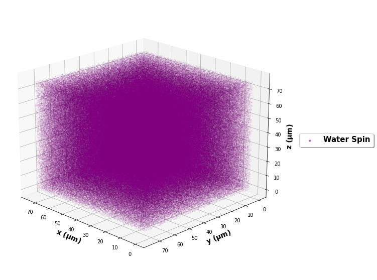
As a first example, let’s simulate isotropic diffusion in an imaging voxel featuring only water. That is,
our imaging voxel will feature no microstructural elements. First, navigate to examples/ under your
simDRIFT installation root directory and run the following command in the console (if you’re outside of the examples/ directory, then you must enter the absolute path to the configuration file):
(simDRIFT) >simDRIFT simulate --configuration qs_isotropic_config.ini
The computation should finish within a minute or two, and the tool will produce a results directory, titled DATE_TIME_simDRIFT_Results/, under which the following files and directories can be found:
trajectories: A directory under which .npy files corresponding to the by-compartment (cells, fiber, water, etc…) and total initial (trajectories_t1m) and final (trajectories_t2p) spin positions are stored. The trajectory files may be useful for generating signals using a different diffusion scheme than the one provided by thediff_schemeargument post-hoc.signals: A directory under which NIfTI files containing the by-compartment and total signals generated fromsimDRIFTare stored.log: A text file that contains a detailed description of the input parameters and a record of the simulation’s executioninput_configuration: A copy of the input INI configuration file so that simulation input parameters may be referenced or simulations may be reproduced in the future.
We can analyze the results using a simple python script:
# Load Data
water_trajectories = np.load(r'PATH_TO_RESULTS/trajectories/water_trajectories_t2p.npy')

# Plot Results
ax = plt.figure(figsize = (10,10)).add_subplot(projection = '3d')
ax.scatter(water_trajectories[1:,0], water_trajectories[1:,1], water_trajectories[1:,2], alpha = 0.05, color = 'purple', s = 1)

# For the figure legend
ax.scatter(water_trajectories[0,0], water_trajectories[0,1], water_trajectories[0,2], alpha = 0.5, color = 'purple', s = 50, label = 'water spin')

ax.view_init(elev = 20., azim = 135)
ax.set_xlabel('x ($\mathbf{\mu m}$)', fontsize = 14, fontweight = 'bold')
ax.set_ylabel('x ($\mathbf{\mu m}$)', fontsize = 14, fontweight = 'bold')
ax.set_zlabel('x ($\mathbf{\mu m}$)', fontsize = 14, fontweight = 'bold')
ax.legend(loc = 'center left', bbox_to_anchor = (1.07, 0.5), fancybox = True,
          shadow = True, prop = {'weight': 'bold', 'size': 15})

plt.show()
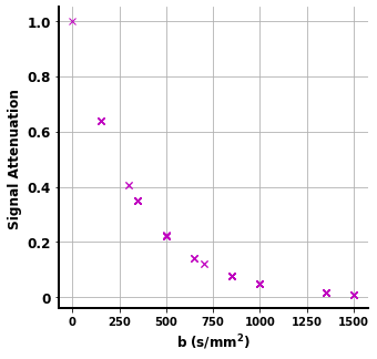
and to check that the simDRIFT reproduced the input water_diffusivity:
# Load Data
bvals = np.loadtxt(r'.../simDRIFT/src/data/bval99')
bvecs = np.loadtxt(r'.../simDRIFT/src/data/bvec99')

water_signal = nb.load(r'.../signals/water_signal.nii').get_fdata()

fig, ax = plt.subplots(figsize = (5,5))
ax.plot(bvals, water_signal, 'mx')
ax.set_yticks([0, 0.2, 0.6, 0.8, 1.0])
ax.set_yticklabels([0, 0.2, 0.6, 0.8, 1.0], fontsize = 12, fontweight = 'bold')
ax.set_xticks([0, 250, 500, 750, 1000, 1250, 1500])
ax.set_xticklabels([0, 250, 500, 750, 1000, 1250, 1500], fontsize = 10, fontweight = 'bold')
ax.spines['top'].set_visible(False)
ax.spines['right'].set_visible(False)
ax.spines['left'].set_linewidth(2)
ax.spines['bottom'].set_linewidth(2)
ax.grid()
ax.set_ylabel('Signal Attenuation', fontsize = 12, fontweight = 'bold')
ax.set_xlabel('b $\mathbf{s / ms^{2}}$', fontsize = 12, fontweight = 'bold')

plt.show()
#Analyze resulst with Dipy
gtab = gradient_table(bvals, bvecs)
tenmodel = dti.TensorModel(gtab)
tenfit = tenmodel.fit(water_signal)

print(1e3 * tenfit.ad, 1e3 * tenfit.rd)
The axial and radial diffusivity of the DTI estimated diffusion tensor are 3.006 \(\mu m^{2} / ms\) and 2.997 \(\mu m^{2} / ms\), confirming
that the diffusion process was indeed isotropic and that simDRIFT faithfully reproduced the input diffusivity here.
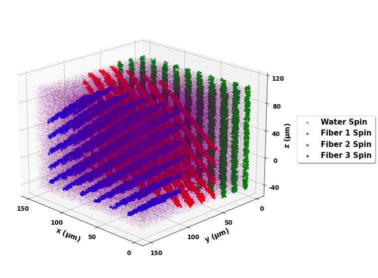
Three Crossing Fibers
Now, let’s simulate a more complicated imaging voxel featuring three crossing fibers with intrinsic diffusivities \(1.0 \mu m^{2} / ms\), \(2.0 \mu m^{2} / ms\), and \(3.0 \mu m^{2} / ms\), and orientations \(0^{\circ}\),
\(45^{\circ}\), \(135^{\circ}\) respectively. To do so, ensure you’re current working directory is still the examples/ directory, and type the following command:
(simDRIFT) >simDRIFT simulate --configuration qs_three_fibers_config.ini
The computation should finish within about five or six minutes.
# Load Data
fiber_1_trajectories = np.load('PATH_TO_RESULTS/trajectories/fiber_1_trajectories_t2p.npy')
fiber_2_trajectories = np.load('PATH_TO_RESULTS/trajectories/fiber_2_trajectories_t2p.npy')
fiber_3_trajectories = np.load('PATH_TO_RESULTS/trajectories/fiber_3_trajectories_t2p.npy')
water_trajectories   = np.load(r'PATH_TO_RESULTS/trajectories/water_trajectories_t1m.npy')

 # Plot Results
ax = plt.figure(figsize = (10,10)).add_subplot(projection = '3d')
ax.scatter(water_trajectories[1:,0], water_trajectories[1:,1], water_trajectories[1:,2], alpha = 0.1, color = 'purple', s = 1)
# For the figure legend
ax.scatter(water_trajectories[0,0], water_trajectories[0,1], water_trajectories[0,2], alpha = 0.5, color = 'purple', label = 'water spin')
ax.scatter(fiber_1_trajectories[:,0], fiber_1_trajectories[:,1], fiber_1_trajectories[:,2], color = 'green', label = 'fiber 1 spin')
ax.scatter(fiber_2_trajectories[:,0], fiber_2_trajectories[:,1], fiber_2_trajectories[:,2], color = 'red',   label = 'fiber 2 spin')
ax.scatter(fiber_3_trajectories[:,0], fiber_3_trajectories[:,1], fiber_3_trajectories[:,2], color = 'blue',  label = 'fiber 3 spin')

ax.view_init(elev = 20., azim = 135)
ax.set_xlabel('x ($\mathbf{\mu m}$)', fontsize = 14, fontweight = 'bold')
ax.set_ylabel('x ($\mathbf{\mu m}$)', fontsize = 14, fontweight = 'bold')
ax.set_zlabel('x ($\mathbf{\mu m}$)', fontsize = 14, fontweight = 'bold')
ax.legend(loc = 'center left', bbox_to_anchor = (1.07, 0.5), fancybox = True,
      shadow = True, prop = {'weight': 'bold', 'size': 15})

plt.show()
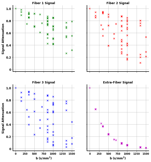
The signal can by analyzed with the below script
# Load Data
bvals = np.loadtxt(r'.../simDRIFT/src/data/bval99')
bvecs = np.loadtxt(r'.../simDRIFT/src/data/bvec99')

fiber_1_signal = nb.load(r'.../signals/fiber_1_signal.nii').get_fdata()
fiber_2_signal = nb.load(r'.../signals/fiber_2_signal.nii').get_fdata()
fiber_3_signal = nb.load(r'.../signals/fiber_3_signal.nii').get_fdata()
water_signal = nb.load(r'.../signals/water_signal.nii').get_fdata()

# Plot Results
fig, axs = plt.subplots(2,2, figsize = (10,10), sharex = True, sharey = True)

axs[0,0].plot(bvals, fiber_1_signal, 'gx')
axs[0,1].plot(bvals, fiber_2_signal, 'rx')
axs[1,0].plot(bvals, fiber_3_signal, 'bx')
axs[1,1].plot(bvals, water_signal,   'mx')

for ax in axs.flatten():
    ax.set_yticks([0, 0.2, 0.6, 0.8, 1.0])
    ax.set_yticklabels([0, 0.2, 0.6, 0.8, 1.0], fontsize = 12, fontweight = 'bold')
    ax.set_xticks([0, 250, 500, 750, 1000, 1250, 1500])
    ax.set_xticklabels([0, 250, 500, 750, 1000, 1250, 1500], fontsize = 10, fontweight = 'bold')
    ax.spines['top'].set_visible(False)
    ax.spines['right'].set_visible(False)
    ax.spines['left'].set_linewidth(2)
    ax.spines['bottom'].set_linewidth(2)
    ax.grid()

axs[0,0].set_ylabel('Signal Attenuation', fontsize = 12, fontweight = 'bold')
axs[1,0].set_ylabel('Signal Attenuation', fontsize = 12, fontweight = 'bold')
axs[1,0].set_xlabel('b $\mathbf{s / ms^{2}}$', fontsize = 12, fontweight = 'bold')
axs[1,1].set_xlabel('b $\mathbf{s / ms^{2}}$', fontsize = 12, fontweight = 'bold')

axs[0,0].set_title('Fiber 1 Signal', fontsize = 12, fontweight = 'bold')
axs[0,1].set_title('Fiber 2 Signal', fontsize = 12, fontweight = 'bold')
axs[1,0].set_title('Fiber 3 Signal', fontsize = 12, fontweight = 'bold')
axs[1,1].set_title('Water Signal', fontsize = 12, fontweight = 'bold')

plt.show()
gtab = gradient_table(bvals, bvecs)
tenmodel = dti.TensorModel(gtab)
tenmodel.fit(water_signal)

tenfit_1 = tenmodel.fit(fiber_1_signal)
tenfit_2 = tenmodel.fit(fiber_2_signal)
tenfit_3 = tenmodel.fit(fiber_3_signal)
tenfit_water = tenmodel.fit(water_signal)

print(1e3 * tenfit_1.ad, 1e3 * tenfit_2.ad, 1e3 * tenfit_3.ad, 1e3 * tenfit_water.ad, 1e3 * tenfit_water.rd)
For the fibers, are estimated axial diffusivities are \(\lambda_{||}^{(1)} = 0.996 \mu m^{2} / ms\), \(\lambda_{||}^{(2)} = 2.007 \mu m^{2} / ms\), \(\lambda_{||}^{(3)} = 2.996 \mu m^{2} / ms\), and for the water, we get that: \(\lambda_{||} = 2.82 \mu m^{2} / ms\) and \(\lambda_{\perp} = 2.73 \mu m^{2} / ms\). The fiber values are exactly in the range that we would expect. Of course, although the water diffusivity is set to \(3.0 \mu m^{2} / ms\), because of the diffusion restricting barriers imposed by the fiber bundles, we can no longer hope to recover this number exactly (at reasonably high fiber densities).
Google Colab
First, open a new Google Colab notebook. Then, nagivate to Edit> Notebook Settings and change the Hardware Accelorator to GPU.
To install Conda, type the following commands.
[ ] #Install Conda
    !pip install -q condacolab
    import condacolab
    condacolab.install()
Now, we create the simDRIFT environment:
[1] #Create Conda Environment
    !conda create -n simDRIFT
To activate the environment:
[2] #Activate Conda Environment
    !source activate simDRIFT
Now that the environment is activated, we can install the dependencies:
[3] #Install Numba
    !conda install numba
     #Install PyTorch
    !pip3 install torch torchvision torchaudio --index-url https://download.pytorch.org/whl/cu117
Now, we install simDRIFT
[4] #Install simDRIFT
    !git clone https://github.com/jacobblum/simDRIFT.git
    !pip install -e simDRIFT
Finally, now that everything is installed let’s run a basic simulation of isotropic diffusion.
[5] !simDRIFT simulate --configuration PATH_TO_CONFIG.INI file